import matplotlib
if not hasattr(matplotlib.RcParams, "_get"):
    matplotlib.RcParams._get = dict.get
Modul 4: Teori#
Pyodide-bemærkning (Python direkte i Browseren)#
Koden i denne Notebook er beregnet til at blive kørt lokalt på din egen computer og ikke direkte i browseren via Pyodide. Årsagen er, at vi bruger scikit-learn til at downloade hele MNIST-datasættet. Dette er en data-tung operation, som involverer download af en stor fil, hvilket ikke umiddelbart understøttes eller er praktisk i et browser-baseret miljø som Pyodide.
Digitale billeder#
import matplotlib.pyplot as plt
import numpy as np
from sklearn.datasets import fetch_openml
# Hent MNIST (784 = 28x28 pixels)
mnist = fetch_openml('mnist_784', version=1, as_frame=False)
X, y = mnist.data, mnist.target.astype('int64')
---------------------------------------------------------------------------
KeyboardInterrupt                         Traceback (most recent call last)
Cell In[1], line 5
      1 import matplotlib.pyplot as plt
      2 import numpy as np
      3 from sklearn.datasets import fetch_openml
      4 # Hent MNIST (784 = 28x28 pixels)
----> 5 mnist = fetch_openml('mnist_784', version=1, as_frame=False)
      6 X, y = mnist.data, mnist.target.astype('int64')

File /usr/local/lib/python3.11/site-packages/sklearn/utils/_param_validation.py:218, in validate_params.<locals>.decorator.<locals>.wrapper(*args, **kwargs)
    212 try:
    213     with config_context(
    214         skip_parameter_validation=(
    215             prefer_skip_nested_validation or global_skip_validation
    216         )
    217     ):
--> 218         return func(*args, **kwargs)
    219 except InvalidParameterError as e:
    220     # When the function is just a wrapper around an estimator, we allow
    221     # the function to delegate validation to the estimator, but we replace
    222     # the name of the estimator by the name of the function in the error
    223     # message to avoid confusion.
    224     msg = re.sub(
    225         r"parameter of \w+ must be",
    226         f"parameter of {func.__qualname__} must be",
    227         str(e),
    228     )

File /usr/local/lib/python3.11/site-packages/sklearn/datasets/_openml.py:1135, in fetch_openml(name, version, data_id, data_home, target_column, cache, return_X_y, as_frame, n_retries, delay, parser, read_csv_kwargs)
   1133 # obtain the data
   1134 url = data_description["url"]
-> 1135 bunch = _download_data_to_bunch(
   1136     url,
   1137     return_sparse,
   1138     data_home,
   1139     as_frame=bool(as_frame),
   1140     openml_columns_info=features_list,
   1141     shape=shape,
   1142     target_columns=target_columns,
   1143     data_columns=data_columns,
   1144     md5_checksum=data_description["md5_checksum"],
   1145     n_retries=n_retries,
   1146     delay=delay,
   1147     parser=parser_,
   1148     read_csv_kwargs=read_csv_kwargs,
   1149 )
   1151 if return_X_y:
   1152     return bunch.data, bunch.target

File /usr/local/lib/python3.11/site-packages/sklearn/datasets/_openml.py:689, in _download_data_to_bunch(url, sparse, data_home, as_frame, openml_columns_info, data_columns, target_columns, shape, md5_checksum, n_retries, delay, parser, read_csv_kwargs)
    685     from pandas.errors import ParserError
    687     no_retry_exception = ParserError
--> 689 X, y, frame, categories = _retry_with_clean_cache(
    690     url, data_home, no_retry_exception
    691 )(_load_arff_response)(
    692     url,
    693     data_home,
    694     parser=parser,
    695     output_type=output_type,
    696     openml_columns_info=features_dict,
    697     feature_names_to_select=data_columns,
    698     target_names_to_select=target_columns,
    699     shape=shape,
    700     md5_checksum=md5_checksum,
    701     n_retries=n_retries,
    702     delay=delay,
    703     read_csv_kwargs=read_csv_kwargs,
    704 )
    706 return Bunch(
    707     data=X,
    708     target=y,
   (...)    712     target_names=target_columns,
    713 )

File /usr/local/lib/python3.11/site-packages/sklearn/datasets/_openml.py:66, in _retry_with_clean_cache.<locals>.decorator.<locals>.wrapper(*args, **kw)
     64     return f(*args, **kw)
     65 try:
---> 66     return f(*args, **kw)
     67 except URLError:
     68     raise

File /usr/local/lib/python3.11/site-packages/sklearn/datasets/_openml.py:554, in _load_arff_response(url, data_home, parser, output_type, openml_columns_info, feature_names_to_select, target_names_to_select, shape, md5_checksum, n_retries, delay, read_csv_kwargs)
    544 arff_params: Dict = dict(
    545     parser=parser,
    546     output_type=output_type,
   (...)    551     read_csv_kwargs=read_csv_kwargs or {},
    552 )
    553 try:
--> 554     X, y, frame, categories = _open_url_and_load_gzip_file(
    555         url, data_home, n_retries, delay, arff_params
    556     )
    557 except Exception as exc:
    558     if parser != "pandas":

File /usr/local/lib/python3.11/site-packages/sklearn/datasets/_openml.py:542, in _load_arff_response.<locals>._open_url_and_load_gzip_file(url, data_home, n_retries, delay, arff_params)
    540 gzip_file = _open_openml_url(url, data_home, n_retries=n_retries, delay=delay)
    541 with closing(gzip_file):
--> 542     return load_arff_from_gzip_file(gzip_file, **arff_params)

File /usr/local/lib/python3.11/site-packages/sklearn/datasets/_arff_parser.py:533, in load_arff_from_gzip_file(gzip_file, parser, output_type, openml_columns_info, feature_names_to_select, target_names_to_select, shape, read_csv_kwargs)
    524     return _liac_arff_parser(
    525         gzip_file,
    526         output_type,
   (...)    530         shape,
    531     )
    532 elif parser == "pandas":
--> 533     return _pandas_arff_parser(
    534         gzip_file,
    535         output_type,
    536         openml_columns_info,
    537         feature_names_to_select,
    538         target_names_to_select,
    539         read_csv_kwargs,
    540     )
    541 else:
    542     raise ValueError(
    543         f"Unknown parser: '{parser}'. Should be 'liac-arff' or 'pandas'."
    544     )

File /usr/local/lib/python3.11/site-packages/sklearn/datasets/_arff_parser.py:404, in _pandas_arff_parser(gzip_file, output_arrays_type, openml_columns_info, feature_names_to_select, target_names_to_select, read_csv_kwargs)
    392 default_read_csv_kwargs = {
    393     "header": None,
    394     "index_col": False,  # always force pandas to not use the first column as index
   (...)    401     "dtype": dtypes_positional,
    402 }
    403 read_csv_kwargs = {**default_read_csv_kwargs, **(read_csv_kwargs or {})}
--> 404 frame = pd.read_csv(gzip_file, **read_csv_kwargs)
    405 try:
    406     # Setting the columns while reading the file will select the N first columns
    407     # and not raise a ParserError. Instead, we set the columns after reading the
    408     # file and raise a ParserError if the number of columns does not match the
    409     # number of columns in the metadata given by OpenML.
    410     frame.columns = [name for name in openml_columns_info]

File /usr/local/lib/python3.11/site-packages/pandas/io/parsers/readers.py:873, in read_csv(filepath_or_buffer, sep, delimiter, header, names, index_col, usecols, dtype, engine, converters, true_values, false_values, skipinitialspace, skiprows, skipfooter, nrows, na_values, keep_default_na, na_filter, skip_blank_lines, parse_dates, date_format, dayfirst, cache_dates, iterator, chunksize, compression, thousands, decimal, lineterminator, quotechar, quoting, doublequote, escapechar, comment, encoding, encoding_errors, dialect, on_bad_lines, low_memory, memory_map, float_precision, storage_options, dtype_backend)
    861 kwds_defaults = _refine_defaults_read(
    862     dialect,
    863     delimiter,
   (...)    869     dtype_backend=dtype_backend,
    870 )
    871 kwds.update(kwds_defaults)
--> 873 return _read(filepath_or_buffer, kwds)

File /usr/local/lib/python3.11/site-packages/pandas/io/parsers/readers.py:306, in _read(filepath_or_buffer, kwds)
    303     return parser
    305 with parser:
--> 306     return parser.read(nrows)

File /usr/local/lib/python3.11/site-packages/pandas/io/parsers/readers.py:1947, in TextFileReader.read(self, nrows)
   1940 nrows = validate_integer("nrows", nrows)
   1941 try:
   1942     # error: "ParserBase" has no attribute "read"
   1943     (
   1944         index,
   1945         columns,
   1946         col_dict,
-> 1947     ) = self._engine.read(  # type: ignore[attr-defined]
   1948         nrows
   1949     )
   1950 except Exception:
   1951     self.close()

File /usr/local/lib/python3.11/site-packages/pandas/io/parsers/c_parser_wrapper.py:215, in CParserWrapper.read(self, nrows)
    213 try:
    214     if self.low_memory:
--> 215         chunks = self._reader.read_low_memory(nrows)
    216         # destructive to chunks
    217         data = _concatenate_chunks(chunks, self.names)

File pandas/_libs/parsers.pyx:832, in pandas._libs.parsers.TextReader.read_low_memory()
--> 832 'Could not get source, probably due dynamically evaluated source code.'

File pandas/_libs/parsers.pyx:911, in pandas._libs.parsers.TextReader._read_rows()
--> 911 'Could not get source, probably due dynamically evaluated source code.'

File pandas/_libs/parsers.pyx:1009, in pandas._libs.parsers.TextReader._convert_column_data()
-> 1009 'Could not get source, probably due dynamically evaluated source code.'

File pandas/_libs/parsers.pyx:1048, in pandas._libs.parsers.TextReader._convert_tokens()
-> 1048 'Could not get source, probably due dynamically evaluated source code.'

File pandas/_libs/parsers.pyx:1145, in pandas._libs.parsers.TextReader._convert_with_dtype()
-> 1145 'Could not get source, probably due dynamically evaluated source code.'

File /usr/local/lib/python3.11/site-packages/pandas/core/dtypes/dtypes.py:531, in CategoricalDtype.construct_array_type(self)
    528     combined_hashed = combine_hash_arrays(iter(cat_array), num_items=len(cat_array))
    529     return np.bitwise_xor.reduce(combined_hashed)
--> 531 def construct_array_type(self) -> type_t[Categorical]:
    532     """
    533     Return the array type associated with this dtype.
    534
   (...)    537     type
    538     """
    539     from pandas import Categorical

KeyboardInterrupt:
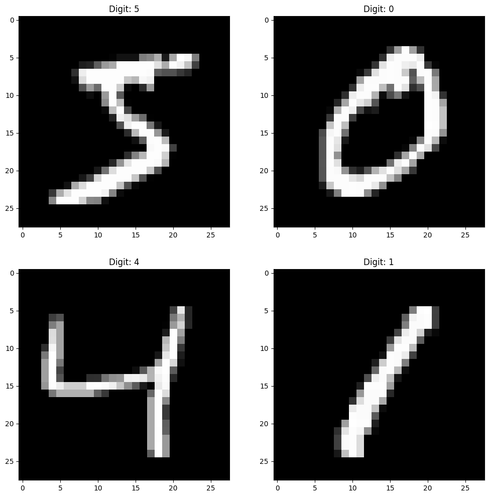
plt.figure(figsize=(12, 12))
plt.subplot(221)
plt.imshow(X[0].reshape(28, 28), cmap='gray')
plt.title(f"Digit: {y[0]}")
plt.subplot(222)
plt.imshow(X[1].reshape(28, 28), cmap='gray')
plt.title(f"Digit: {y[1]}")
plt.subplot(223)
plt.imshow(X[2].reshape(28, 28), cmap='gray')
plt.title(f"Digit: {y[2]}")
plt.subplot(224)
plt.imshow(X[3].reshape(28, 28), cmap='gray')
plt.title(f"Digit: {y[3]}")
# vis grafen
plt.show()
Vektorfunktioner#
Lad \(d,k \in \mathbb{N}\). En vektorfunktion af flere variable er en funktion af formen
Altså har en vektorfunktion \(\pmb{f} = \pmb{x} \mapsto \pmb{f}(\pmb{x})\):
Input (domænet): vektorer \(\pmb{x}\) i \(\mathbb{R}^d\)
Output (kodomænet): vektorer \(\pmb{f}(\pmb{x})\) i \(\mathbb{R}^k\)
Input \(\pmb{x}_0\)#
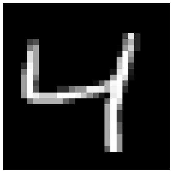
# Vis det tredje billede fra træningssættet
x0 = X[2].reshape(28, 28)
plt.figure(figsize=(7, 7))
plt.imshow(x0, cmap='gray')
plt.axis('off')
plt.show()
Output \(\pmb{f}(\pmb{x}_0)\)#
Output:
"Dette er cifret 4"
Ideelt output:
Dette betyder: "100% sikker på, at dette er cifret 4"
Mere realistisk output:
Dette betyder: "87% sikker på, at dette er cifret 4. Lille sandsynlighed (3%) for, at det er 1 eller 7."
Under alle omstændigheder: Outputtet er en vektor af sandsynligheder i \(\mathbb{R}^{10}\). Derfor er \(\operatorname{co\text{-}dom}(\pmb{f})=\mathbb{R}^{10}\).
Hvad med inputtet?#
Det er faktisk en matrix på størrelse 28x28:
Men det er ikke umiddelbart en (søjle)vektor!
Vi kan gøre den om til en vektor ved at stakke billedets rækker oven på hinanden. Dette kaldes flattening (udfladning) af billedet i Python.
# Udskriv som søjle med 784 tal
print("\nSøjle-repræsentation af billedet (784 tal):")
x0.reshape(784,1)
Søjle-repræsentation af billedet (784 tal):
array([[ 0],
[ 0],
[ 0],
[ 0],
[ 0],
[ 0],
[ 0],
[ 0],
[ 0],
[ 0],
[ 0],
[ 0],
[ 0],
[ 0],
[ 0],
[ 0],
[ 0],
[ 0],
[ 0],
[ 0],
[ 0],
[ 0],
[ 0],
[ 0],
[ 0],
[ 0],
[ 0],
[ 0],
[ 0],
[ 0],
[ 0],
[ 0],
[ 0],
[ 0],
[ 0],
[ 0],
[ 0],
[ 0],
[ 0],
[ 0],
[ 0],
[ 0],
[ 0],
[ 0],
[ 0],
[ 0],
[ 0],
[ 0],
[ 0],
[ 0],
[ 0],
[ 0],
[ 0],
[ 0],
[ 0],
[ 0],
[ 0],
[ 0],
[ 0],
[ 0],
[ 0],
[ 0],
[ 0],
[ 0],
[ 0],
[ 0],
[ 0],
[ 0],
[ 0],
[ 0],
[ 0],
[ 0],
[ 0],
[ 0],
[ 0],
[ 0],
[ 0],
[ 0],
[ 0],
[ 0],
[ 0],
[ 0],
[ 0],
[ 0],
[ 0],
[ 0],
[ 0],
[ 0],
[ 0],
[ 0],
[ 0],
[ 0],
[ 0],
[ 0],
[ 0],
[ 0],
[ 0],
[ 0],
[ 0],
[ 0],
[ 0],
[ 0],
[ 0],
[ 0],
[ 0],
[ 0],
[ 0],
[ 0],
[ 0],
[ 0],
[ 0],
[ 0],
[ 0],
[ 0],
[ 0],
[ 0],
[ 0],
[ 0],
[ 0],
[ 0],
[ 0],
[ 0],
[ 0],
[ 0],
[ 0],
[ 0],
[ 0],
[ 0],
[ 0],
[ 0],
[ 0],
[ 0],
[ 0],
[ 0],
[ 0],
[ 0],
[ 0],
[ 0],
[ 0],
[ 0],
[ 0],
[ 0],
[ 0],
[ 0],
[ 0],
[ 0],
[ 0],
[ 0],
[ 0],
[ 0],
[ 0],
[ 0],
[ 0],
[ 0],
[ 0],
[ 0],
[ 0],
[ 0],
[ 0],
[ 0],
[ 67],
[232],
[ 39],
[ 0],
[ 0],
[ 0],
[ 0],
[ 0],
[ 0],
[ 0],
[ 0],
[ 0],
[ 62],
[ 81],
[ 0],
[ 0],
[ 0],
[ 0],
[ 0],
[ 0],
[ 0],
[ 0],
[ 0],
[ 0],
[ 0],
[ 0],
[ 0],
[ 0],
[120],
[180],
[ 39],
[ 0],
[ 0],
[ 0],
[ 0],
[ 0],
[ 0],
[ 0],
[ 0],
[ 0],
[126],
[163],
[ 0],
[ 0],
[ 0],
[ 0],
[ 0],
[ 0],
[ 0],
[ 0],
[ 0],
[ 0],
[ 0],
[ 0],
[ 0],
[ 2],
[153],
[210],
[ 40],
[ 0],
[ 0],
[ 0],
[ 0],
[ 0],
[ 0],
[ 0],
[ 0],
[ 0],
[220],
[163],
[ 0],
[ 0],
[ 0],
[ 0],
[ 0],
[ 0],
[ 0],
[ 0],
[ 0],
[ 0],
[ 0],
[ 0],
[ 0],
[ 27],
[254],
[162],
[ 0],
[ 0],
[ 0],
[ 0],
[ 0],
[ 0],
[ 0],
[ 0],
[ 0],
[ 0],
[222],
[163],
[ 0],
[ 0],
[ 0],
[ 0],
[ 0],
[ 0],
[ 0],
[ 0],
[ 0],
[ 0],
[ 0],
[ 0],
[ 0],
[183],
[254],
[125],
[ 0],
[ 0],
[ 0],
[ 0],
[ 0],
[ 0],
[ 0],
[ 0],
[ 0],
[ 46],
[245],
[163],
[ 0],
[ 0],
[ 0],
[ 0],
[ 0],
[ 0],
[ 0],
[ 0],
[ 0],
[ 0],
[ 0],
[ 0],
[ 0],
[198],
[254],
[ 56],
[ 0],
[ 0],
[ 0],
[ 0],
[ 0],
[ 0],
[ 0],
[ 0],
[ 0],
[120],
[254],
[163],
[ 0],
[ 0],
[ 0],
[ 0],
[ 0],
[ 0],
[ 0],
[ 0],
[ 0],
[ 0],
[ 0],
[ 0],
[ 23],
[231],
[254],
[ 29],
[ 0],
[ 0],
[ 0],
[ 0],
[ 0],
[ 0],
[ 0],
[ 0],
[ 0],
[159],
[254],
[120],
[ 0],
[ 0],
[ 0],
[ 0],
[ 0],
[ 0],
[ 0],
[ 0],
[ 0],
[ 0],
[ 0],
[ 0],
[163],
[254],
[216],
[ 16],
[ 0],
[ 0],
[ 0],
[ 0],
[ 0],
[ 0],
[ 0],
[ 0],
[ 0],
[159],
[254],
[ 67],
[ 0],
[ 0],
[ 0],
[ 0],
[ 0],
[ 0],
[ 0],
[ 0],
[ 0],
[ 14],
[ 86],
[178],
[248],
[254],
[ 91],
[ 0],
[ 0],
[ 0],
[ 0],
[ 0],
[ 0],
[ 0],
[ 0],
[ 0],
[ 0],
[159],
[254],
[ 85],
[ 0],
[ 0],
[ 0],
[ 47],
[ 49],
[116],
[144],
[150],
[241],
[243],
[234],
[179],
[241],
[252],
[ 40],
[ 0],
[ 0],
[ 0],
[ 0],
[ 0],
[ 0],
[ 0],
[ 0],
[ 0],
[ 0],
[150],
[253],
[237],
[207],
[207],
[207],
[253],
[254],
[250],
[240],
[198],
[143],
[ 91],
[ 28],
[ 5],
[233],
[250],
[ 0],
[ 0],
[ 0],
[ 0],
[ 0],
[ 0],
[ 0],
[ 0],
[ 0],
[ 0],
[ 0],
[ 0],
[119],
[177],
[177],
[177],
[177],
[177],
[ 98],
[ 56],
[ 0],
[ 0],
[ 0],
[ 0],
[ 0],
[102],
[254],
[220],
[ 0],
[ 0],
[ 0],
[ 0],
[ 0],
[ 0],
[ 0],
[ 0],
[ 0],
[ 0],
[ 0],
[ 0],
[ 0],
[ 0],
[ 0],
[ 0],
[ 0],
[ 0],
[ 0],
[ 0],
[ 0],
[ 0],
[ 0],
[ 0],
[ 0],
[169],
[254],
[137],
[ 0],
[ 0],
[ 0],
[ 0],
[ 0],
[ 0],
[ 0],
[ 0],
[ 0],
[ 0],
[ 0],
[ 0],
[ 0],
[ 0],
[ 0],
[ 0],
[ 0],
[ 0],
[ 0],
[ 0],
[ 0],
[ 0],
[ 0],
[ 0],
[ 0],
[169],
[254],
[ 57],
[ 0],
[ 0],
[ 0],
[ 0],
[ 0],
[ 0],
[ 0],
[ 0],
[ 0],
[ 0],
[ 0],
[ 0],
[ 0],
[ 0],
[ 0],
[ 0],
[ 0],
[ 0],
[ 0],
[ 0],
[ 0],
[ 0],
[ 0],
[ 0],
[ 0],
[169],
[254],
[ 57],
[ 0],
[ 0],
[ 0],
[ 0],
[ 0],
[ 0],
[ 0],
[ 0],
[ 0],
[ 0],
[ 0],
[ 0],
[ 0],
[ 0],
[ 0],
[ 0],
[ 0],
[ 0],
[ 0],
[ 0],
[ 0],
[ 0],
[ 0],
[ 0],
[ 0],
[169],
[255],
[ 94],
[ 0],
[ 0],
[ 0],
[ 0],
[ 0],
[ 0],
[ 0],
[ 0],
[ 0],
[ 0],
[ 0],
[ 0],
[ 0],
[ 0],
[ 0],
[ 0],
[ 0],
[ 0],
[ 0],
[ 0],
[ 0],
[ 0],
[ 0],
[ 0],
[ 0],
[169],
[254],
[ 96],
[ 0],
[ 0],
[ 0],
[ 0],
[ 0],
[ 0],
[ 0],
[ 0],
[ 0],
[ 0],
[ 0],
[ 0],
[ 0],
[ 0],
[ 0],
[ 0],
[ 0],
[ 0],
[ 0],
[ 0],
[ 0],
[ 0],
[ 0],
[ 0],
[ 0],
[169],
[254],
[153],
[ 0],
[ 0],
[ 0],
[ 0],
[ 0],
[ 0],
[ 0],
[ 0],
[ 0],
[ 0],
[ 0],
[ 0],
[ 0],
[ 0],
[ 0],
[ 0],
[ 0],
[ 0],
[ 0],
[ 0],
[ 0],
[ 0],
[ 0],
[ 0],
[ 0],
[169],
[255],
[153],
[ 0],
[ 0],
[ 0],
[ 0],
[ 0],
[ 0],
[ 0],
[ 0],
[ 0],
[ 0],
[ 0],
[ 0],
[ 0],
[ 0],
[ 0],
[ 0],
[ 0],
[ 0],
[ 0],
[ 0],
[ 0],
[ 0],
[ 0],
[ 0],
[ 0],
[ 96],
[254],
[153],
[ 0],
[ 0],
[ 0],
[ 0],
[ 0],
[ 0],
[ 0],
[ 0],
[ 0],
[ 0],
[ 0],
[ 0],
[ 0],
[ 0],
[ 0],
[ 0],
[ 0],
[ 0],
[ 0],
[ 0],
[ 0],
[ 0],
[ 0],
[ 0],
[ 0],
[ 0],
[ 0],
[ 0],
[ 0],
[ 0],
[ 0],
[ 0],
[ 0],
[ 0],
[ 0],
[ 0],
[ 0],
[ 0],
[ 0],
[ 0],
[ 0],
[ 0],
[ 0],
[ 0],
[ 0],
[ 0],
[ 0],
[ 0],
[ 0],
[ 0],
[ 0],
[ 0],
[ 0],
[ 0],
[ 0],
[ 0],
[ 0],
[ 0],
[ 0],
[ 0],
[ 0],
[ 0],
[ 0],
[ 0],
[ 0],
[ 0],
[ 0],
[ 0],
[ 0],
[ 0],
[ 0],
[ 0],
[ 0],
[ 0],
[ 0],
[ 0],
[ 0],
[ 0],
[ 0],
[ 0],
[ 0],
[ 0],
[ 0],
[ 0],
[ 0],
[ 0],
[ 0],
[ 0],
[ 0],
[ 0],
[ 0],
[ 0]])
Så vi kan tænke på inputtet som vektorer i \(\mathbb{R}^{784}\)! Det vil sige
En AI funktion#
AI’en er en vektorfunktion med \(d=784\), \(k=10\).
I maskinlæring kaldes funktionen for en model, og den specifikke AI-funktion afhænger typisk af tusindvis eller millioner af parametre (kaldet vægte). For hvert sæt af parametre/vægte får vi en ny AI-funktion. Sådanne funktioner (også dybe neurale netværk) er ikke særligt komplicerede, men ofte lange at skrive eksplicit. De er bygget af
Sammensætning af simple vektorfunktioner \(\pmb{g} \circ \pmb{h}\)
De simple funktioner er normalt kun: 1. Affine vektorfunktioner \(\pmb{x} \mapsto A \pmb{x} + \pmb{b}\) (elementerne i matrixen \(A\) og vektoren \(\pmb{b}\) er parametrene/vægtene) 2. En ikke-lineær aktiveringsfunktion, fx ReLU.
Antallet af sammensætninger \(\pmb{g}_1 \circ \pmb{g}_2 \circ \pmb{g}_3 \circ \cdots \circ \pmb{g}_N\) beskriver netværkets dybde.
Neurale netværk#
Hvordan ser disse “AI-funktioner” ud?
Generel notation for et feedforward ReLU-netværk#
Et feedforward-netværk beregner outputtet ved sekventielt at føre input gennem en række lag. For hvert lag \(\ell\) beregnes først en pre-aktivering (også kaldet logits), \(z^{(\ell)}\), efterfulgt af en aktivering (eller hidden state), \(h^{(\ell)}\).
hvor
\(h^{(0)}\) er input-vektoren \(x\).
\(W_\ell \in \mathbb{R}^{n_\ell \times n_{\ell-1}}\) er vægtmatricen for lag \(\ell\).
\(b_\ell \in \mathbb{R}^{n_\ell}\) er bias-vektoren.
\(\sigma:\mathbb{R}\to\mathbb{R}\) er en ikke-lineær aktiveringsfunktion (anvendt koordinatvis) typisk ReLU:
\(n_0=d\) er inputdimensionen, \(n_L=k\) outputdimensionen.
Vi siger kort at netværket er af formen \(n_0 \to n_1 \to \cdots \to n_L\).
Netværkets samlede funktion \(\Phi: \mathbb{R}^d \to \mathbb{R}^k\) giver det endelige output:
idet sidste lag her er lineært (uden ReLU-aktivering).

Shallow netværk (ét skjult lag med L=2)#
For et shallow netværk \(\Phi:\mathbb{R}^2\to\mathbb{R}\) med ét skjult lag af størrelse \(n\):
hvor
\(x \in \mathbb{R}^2\),
\(W_1 \in \mathbb{R}^{n\times 2},\ b_1 \in \mathbb{R}^{n},\)
\(W_2 \in \mathbb{R}^{1\times n},\ b_2 \in \mathbb{R}.\)
Illustration af lagene:
Hvert ReLU-lag opdeler rummet i lineære regioner bestemt af ligningerne \( (W_\ell h^{(\ell-1)} + b_\ell)_i = 0 \), så \(\Phi\) er en stykkevist lineær funktion på \(\mathbb{R}^d\).
Generel formel for et ReLU-netværk med \(L=3\)#
Vi betragter en funktion
defineret som et fuldt forbundet netværk med to skjulte lag:
hvor \(n_0 = d\), \(n_3 = k\), og
\(W_1 \in \mathbb{R}^{n_1\times n_0},\ b_1\in\mathbb{R}^{n_1}\)
\(W_2 \in \mathbb{R}^{n_2\times n_1},\ b_2\in\mathbb{R}^{n_2}\)
\(W_3 \in \mathbb{R}^{n_3\times n_2},\ b_3\in\mathbb{R}^{n_3}\)
Det samlede funktionsudtryk bliver:
Eksempel: For et konkret netværk med to inputvariabler og ét output af formen \(2 \to n_1 \to n_2 \to 1\):
hvor dimensionerne er
Netværk og træning direkte i SKLearn#
Vi skal finde en “AI-funktion”
der “bedst”-muligt kan klassificere et billede af et håndskrevet ciffer.
I koden nedenfor opbygges denne som et ReLU-netværk med to skjulte lag, hvilket giver en samlet dybde på \(L=3\). Formen af netværket er \(784 \to 256 \to 128 \to 10\). Altså er vægt-matricerne af størrelse
from sklearn.model_selection import train_test_split
from sklearn.neural_network import MLPClassifier

# Normaliser til [0,1]
X = X / 255.0

X_train, X_test, y_train, y_test = train_test_split(
    X, y, test_size=1/7, random_state=42
)

# DNN med samme “størrelse” som PyTorch-eksemplet
clf = MLPClassifier(
    hidden_layer_sizes=(256, 128),  # to skjulte lag
    activation='relu',
    solver='adam',
    batch_size=64,
    learning_rate_init=1e-3,
    max_iter=6,
    verbose=True
)
Netværkets størrelse#
Hvor mange parametre er der?
Svar#
Det samlede antal parametre for netværket er:
Lag 1: (784 input × 256 neuroner) + 256 bias = 200.704 + 256 = 200.960
Lag 2: (256 input × 128 neuroner) + 128 bias = 32.768 + 128 = 32.896
Lag 3: (128 input × 10 neuroner) + 10 bias = 1.280 + 10 = 1.290
I alt: 200.960 + 32.896 + 1.290 = 235.146
Træning via SKLearn#
Vi finder de optimale værdier for alle parametrene i \(Phi-\)funktionen ved at træne modellen med fit-metoden:
# Træn
clf.fit(X_train, y_train)
Iteration 1, loss = 0.22757620
Iteration 2, loss = 0.08920455
Iteration 3, loss = 0.05955793
Iteration 4, loss = 0.04347159
Iteration 5, loss = 0.03397271
Iteration 6, loss = 0.02918372
/home/jakle/Python/envs/intermat/lib/python3.10/site-packages/sklearn/neural_network/_multilayer_perceptron.py:781: ConvergenceWarning: Stochastic Optimizer: Maximum iterations (6) reached and the optimization hasn't converged yet.
  warnings.warn(
MLPClassifier(batch_size=64, hidden_layer_sizes=(256, 128), max_iter=6,
              verbose=True)
In a Jupyter environment, please rerun this cell to show the HTML representation or trust the notebook. On GitHub, the HTML representation is unable to render, please try loading this page with nbviewer.org.
Parameters
| hidden_layer_sizes | (256, ...) | |
| activation | 'relu' | |
| solver | 'adam' | |
| alpha | 0.0001 | |
| batch_size | 64 | |
| learning_rate | 'constant' | |
| learning_rate_init | 0.001 | |
| power_t | 0.5 | |
| max_iter | 6 | |
| shuffle | True | |
| random_state | None | |
| tol | 0.0001 | |
| verbose | True | |
| warm_start | False | |
| momentum | 0.9 | |
| nesterovs_momentum | True | |
| early_stopping | False | |
| validation_fraction | 0.1 | |
| beta_1 | 0.9 | |
| beta_2 | 0.999 | |
| epsilon | 1e-08 | |
| n_iter_no_change | 10 | |
| max_fun | 15000 |
Forudsigelse på et enkelt billede#
Denne funktion kan vi nu bruge på et enkelt input-billede for at få en forudsigelse. Lad os tage et enkelt billede fra vores testsæt og se, hvad modellen forudsiger.
image_index = 2 # Vælg et billede (input)
input_image = X_test[image_index:image_index+1] # Format (1, 784)
true_label = y_test[image_index]

probability_vector = clf.predict_proba(input_image) # Få sandsynlighedsvektoren
predicted_label = clf.predict(input_image) # Lav forudsigelse

print(input_image)
print(true_label)
print(probability_vector)
print(predicted_label)
[[0.         0.         0.         0.         0.         0.
  0.         0.         0.         0.         0.         0.
  0.         0.         0.         0.         0.         0.
  0.         0.         0.         0.         0.         0.
  0.         0.         0.         0.         0.         0.
  0.         0.         0.         0.         0.         0.
  0.         0.         0.         0.         0.         0.
  0.         0.         0.         0.         0.         0.
  0.         0.         0.         0.         0.         0.
  0.         0.         0.         0.         0.         0.
  0.         0.         0.         0.         0.         0.
  0.         0.         0.         0.         0.         0.
  0.         0.         0.         0.         0.         0.
  0.         0.         0.         0.         0.         0.
  0.         0.         0.         0.         0.         0.
  0.         0.         0.         0.         0.         0.
  0.         0.         0.         0.         0.         0.
  0.         0.         0.         0.         0.         0.
  0.         0.         0.         0.         0.         0.
  0.         0.         0.         0.         0.         0.
  0.         0.         0.         0.         0.         0.
  0.         0.         0.         0.         0.         0.
  0.         0.         0.         0.         0.         0.
  0.         0.         0.         0.         0.         0.
  0.         0.         0.         0.         0.         0.
  0.         0.         0.         0.         0.         0.
  0.61960784 0.90588235 0.14901961 0.         0.         0.
  0.         0.         0.         0.         0.         0.
  0.         0.         0.         0.         0.         0.
  0.         0.         0.         0.02745098 0.25490196 0.56862745
  0.56862745 0.34509804 0.         0.05490196 0.83137255 0.99215686
  0.28235294 0.         0.         0.         0.         0.
  0.         0.         0.         0.         0.         0.
  0.         0.         0.         0.         0.09019608 0.14509804
  0.25882353 0.7254902  0.99215686 0.9372549  0.91372549 0.99215686
  0.59607843 0.45490196 0.99215686 0.80784314 0.10980392 0.
  0.         0.         0.         0.         0.         0.
  0.         0.         0.         0.         0.         0.
  0.         0.06666667 0.87058824 0.99215686 0.99215686 0.9372549
  0.80392157 0.27058824 0.14509804 0.64705882 0.99607843 0.99215686
  0.89803922 0.10980392 0.         0.         0.         0.
  0.         0.         0.         0.         0.         0.
  0.         0.         0.         0.         0.         0.0745098
  0.90196078 0.99215686 0.99215686 0.48235294 0.         0.
  0.         0.58823529 0.99607843 0.81176471 0.24313725 0.
  0.         0.         0.         0.         0.         0.
  0.         0.         0.         0.         0.         0.
  0.         0.         0.         0.         0.14901961 0.60392157
  0.99215686 0.78823529 0.19215686 0.         0.46666667 0.98431373
  0.98431373 0.30588235 0.         0.         0.         0.
  0.         0.         0.         0.         0.         0.
  0.         0.         0.         0.         0.         0.
  0.         0.         0.         0.03921569 0.76470588 0.99215686
  0.92941176 0.80784314 0.97647059 0.99215686 0.56470588 0.
  0.         0.         0.         0.         0.         0.
  0.         0.         0.         0.         0.         0.
  0.         0.         0.         0.         0.         0.
  0.         0.         0.10196078 0.50196078 0.92156863 0.99215686
  0.99215686 0.99215686 0.90196078 0.38431373 0.14509804 0.
  0.         0.         0.         0.         0.         0.
  0.         0.         0.         0.         0.         0.
  0.         0.         0.         0.         0.         0.
  0.         0.         0.38039216 0.99215686 0.99215686 0.99215686
  0.99607843 0.99215686 0.9372549  0.58431373 0.12156863 0.
  0.         0.         0.         0.         0.         0.
  0.         0.         0.         0.         0.         0.
  0.         0.         0.         0.         0.         0.
  0.56078431 0.99215686 0.78823529 0.06666667 0.29411765 0.51764706
  0.81176471 0.99215686 0.84705882 0.11372549 0.         0.
  0.         0.         0.         0.         0.         0.
  0.         0.         0.         0.         0.         0.
  0.         0.         0.         0.1372549  0.90196078 0.99607843
  0.54509804 0.         0.         0.         0.07058824 0.56470588
  0.98431373 0.8627451  0.12156863 0.         0.         0.
  0.         0.         0.         0.         0.         0.
  0.         0.         0.         0.         0.         0.
  0.         0.         0.80784314 0.99215686 0.09411765 0.
  0.         0.         0.         0.         0.66666667 0.99215686
  0.69019608 0.01568627 0.         0.         0.         0.
  0.         0.         0.         0.         0.         0.
  0.         0.         0.         0.         0.         0.
  0.50980392 0.99215686 0.38823529 0.         0.         0.
  0.         0.         0.09019608 0.78039216 0.99215686 0.14117647
  0.         0.         0.         0.         0.         0.
  0.         0.         0.         0.         0.         0.
  0.         0.         0.         0.         0.27058824 0.96862745
  0.64705882 0.64313725 0.         0.         0.         0.
  0.         0.28627451 0.99215686 0.45882353 0.         0.
  0.         0.         0.         0.         0.         0.
  0.         0.         0.         0.         0.         0.
  0.         0.         0.         0.85490196 0.99215686 0.99215686
  0.11764706 0.         0.         0.         0.         0.28627451
  0.99215686 0.61176471 0.         0.         0.         0.
  0.         0.         0.         0.         0.         0.
  0.         0.         0.         0.         0.         0.
  0.         0.38431373 0.83137255 0.99215686 0.8745098  0.3254902
  0.         0.         0.         0.07058824 0.85098039 0.90588235
  0.07058824 0.         0.         0.         0.         0.
  0.         0.         0.         0.         0.         0.
  0.         0.         0.         0.         0.         0.
  0.28627451 0.98039216 0.99607843 0.88627451 0.30980392 0.
  0.         0.23529412 0.95686275 0.86666667 0.0627451  0.
  0.         0.         0.         0.         0.         0.
  0.         0.         0.         0.         0.         0.
  0.         0.         0.         0.         0.         0.13333333
  0.99607843 0.99215686 0.83921569 0.30980392 0.         0.28627451
  0.99215686 0.43529412 0.         0.         0.         0.
  0.         0.         0.         0.         0.         0.
  0.         0.         0.         0.         0.         0.
  0.         0.         0.         0.         0.36470588 0.99215686
  0.99215686 0.97647059 0.78823529 0.81568627 0.99215686 0.14117647
  0.         0.         0.         0.         0.         0.
  0.         0.         0.         0.         0.         0.
  0.         0.         0.         0.         0.         0.
  0.         0.         0.00392157 0.31764706 0.81176471 0.99215686
  0.99215686 0.85490196 0.36078431 0.00784314 0.         0.
  0.         0.         0.         0.         0.         0.
  0.         0.         0.         0.         0.         0.
  0.         0.         0.         0.         0.         0.
  0.         0.         0.         0.         0.         0.
  0.         0.         0.         0.         0.         0.
  0.         0.         0.         0.         0.         0.
  0.         0.         0.         0.         0.         0.
  0.         0.         0.         0.         0.         0.
  0.         0.         0.         0.         0.         0.
  0.         0.         0.         0.         0.         0.
  0.         0.         0.         0.         0.         0.
  0.         0.         0.         0.         0.         0.
  0.         0.         0.         0.         0.         0.
  0.         0.         0.         0.         0.         0.
  0.         0.         0.         0.        ]]
8
[[7.08580512e-05 2.61484819e-04 1.44964793e-05 1.17057312e-03
  1.67150883e-05 5.34671916e-02 4.29566890e-01 8.57747096e-06
  5.14443444e-01 9.79769433e-04]]
[8]
Total forudsigelse#
Den samlede procentandel af billeder i testsættet, som modellen klassificerede korrekt kan findes ved:
# Samlet evaluering
print("Test accuracy:", clf.score(X_test, y_test))
Test accuracy: 0.9778
Visualisering af forudsigelser#
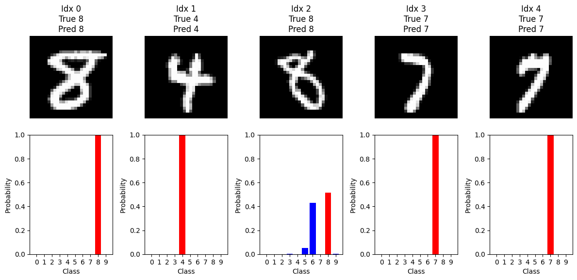
For at få en bedre fornemmelse af, hvordan modellen opfører sig, kan vi visualisere dens forudsigelser på enkelte billeder fra testsættet. Nedenstående funktion plotter billedet, den korrekte label, den forudsagte label og et søjlediagram over de forudsagte sandsynligheder for hver klasse. Dette er nyttigt for at se, hvornår modellen er sikker, og hvornår den er i tvivl.
def show_images_with_mlp_probabilities(clf, X_test, y_test, X_test_orig,
                                       num_images=5, only_incorrect=False,
                                       image_shape=(8,8)):
    # Predict full test set
    pred_labels = clf.predict(X_test)
    probas = clf.predict_proba(X_test)

    # Select indices
    all_indices = np.arange(len(X_test))
    if only_incorrect:
        indices = all_indices[pred_labels != y_test][:num_images]
    else:
        indices = all_indices[:num_images]

    plt.figure(figsize=(12, 6))

    for i, idx in enumerate(indices):
        # --- Image plot ---
        plt.subplot(2, num_images, i + 1)
        img = X_test_orig[idx].reshape(image_shape)
        plt.imshow(img, cmap='gray')
        plt.title(f"Idx {idx}\nTrue {y_test[idx]}\nPred {pred_labels[idx]}")
        plt.axis('off')

        # --- Probability distribution ---
        plt.subplot(2, num_images, num_images + i + 1)

        p = probas[idx]

        classes = np.arange(len(p))
        colors = [
            "red" if c == y_test[idx] else
            ("green" if c == pred_labels[idx] else "blue")
            for c in classes
        ]

        plt.bar(classes, p, color=colors)
        plt.xticks(classes)
        plt.ylim(0, 1)
        plt.xlabel("Class")
        plt.ylabel("Probability")

    plt.tight_layout()
    plt.show()

show_images_with_mlp_probabilities(
    clf,
    X_test,
    y_test,
    X_test_orig=X_test,
    only_incorrect=False,
    num_images=5,
    image_shape=(28,28)
)
show_images_with_mlp_probabilities(
    clf,
    X_test,
    y_test,
    X_test_orig=X_test,
    only_incorrect=True,
    num_images=5,
    image_shape=(28,28)
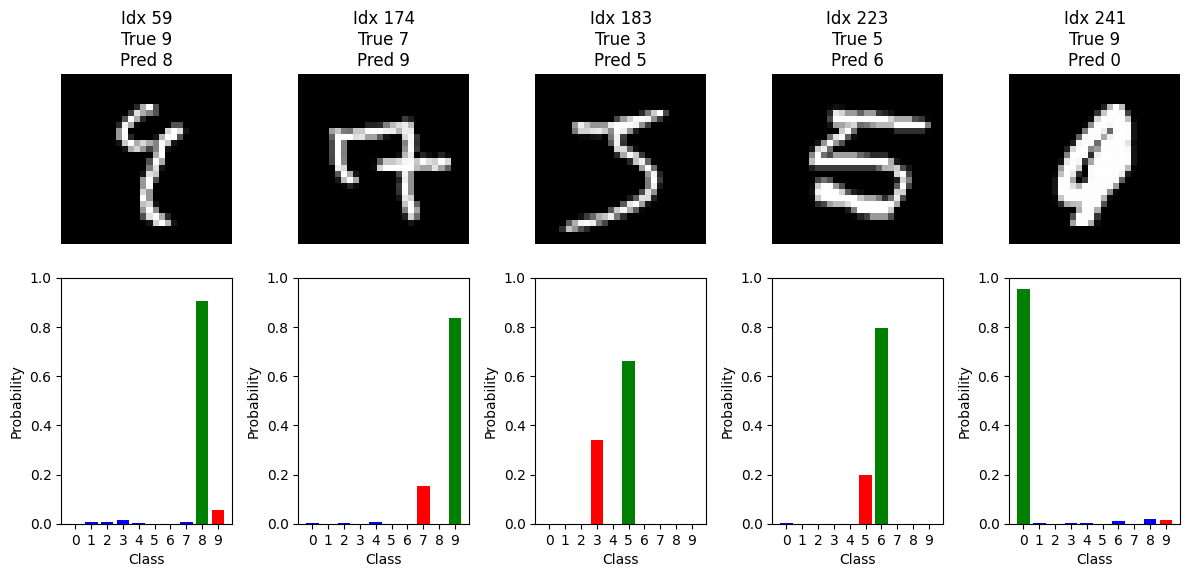
)